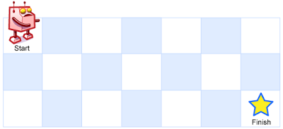
Unique Paths in Python with Time Complexity Analysis

A robot is located at the top-left corner of a n x m grid (marked 'Start' in the diagram below).

The robot can only move either down or right at any moment of time. The robot is trying to reach the bottom-right corner of the grid (marked 'Finish' in the diagram below).

Now consider obstacles are placed in some of the grid's cells. How many unique paths would there be?

An obstacle and empty space is marked as 1 and 0 respectively in the grid.

Note: n and m will be at most 100.

It is guaranteed that the answer can be represented as a 32-bit integer.

Example 1:

Input:
[
  [0,0,0],
  [0,1,0],
  [0,0,0]
]
Output: 2
Explanation:
There is one obstacle in the middle of the 3x3 grid above.
There are two ways to reach the bottom-right corner:
1. Right -> Right -> Down -> Down
2. Down -> Down -> Right -> Right

Understanding the Problem

The core challenge of this problem is to find the number of unique paths from the top-left corner to the bottom-right corner of a grid, considering that some cells may contain obstacles. The robot can only move right or down.

This problem is significant in robotics and pathfinding algorithms, where determining the optimal path in a grid with obstacles is crucial. A common pitfall is not accounting for the obstacles correctly, which can lead to incorrect path counts.

Approach

To solve this problem, we can use dynamic programming. The idea is to create a 2D array `dp` where `dp[i][j]` represents the number of unique paths to reach cell `(i, j)`.

Naive Solution

A naive solution would involve recursively exploring all possible paths, but this approach is not optimal due to its exponential time complexity.

Optimized Solution

We can optimize the solution using dynamic programming:

Initialize a 2D array `dp` with the same dimensions as the grid.
If the starting cell has an obstacle, return 0 immediately.
Set `dp[0][0]` to 1 (starting point).
Iterate through the grid and update the `dp` array based on the values from the top and left cells, considering obstacles.

Algorithm

Here is a step-by-step breakdown of the dynamic programming approach:

Create a 2D array `dp` with dimensions `n x m` initialized to 0.
If the starting cell `grid[0][0]` is 1, return 0 (no paths possible).
Set `dp[0][0]` to 1.
Iterate through each cell in the grid:

If the cell is an obstacle, set `dp[i][j]` to 0.
Otherwise, set `dp[i][j]` to the sum of `dp[i-1][j]` (top cell) and `dp[i][j-1]` (left cell), if they exist.

Return `dp[n-1][m-1]` as the result.

Code Implementation

def unique_paths_with_obstacles(grid):
    # Get the dimensions of the grid
    n = len(grid)
    m = len(grid[0])
    
    # If the starting point or the ending point is an obstacle, return 0
    if grid[0][0] == 1 or grid[n-1][m-1] == 1:
        return 0
    
    # Initialize the dp array with zeros
    dp = [[0] * m for _ in range(n)]
    
    # Starting point
    dp[0][0] = 1
    
    # Fill the dp array
    for i in range(n):
        for j in range(m):
            if grid[i][j] == 1:
                dp[i][j] = 0
            else:
                if i > 0:
                    dp[i][j] += dp[i-1][j]
                if j > 0:
                    dp[i][j] += dp[i][j-1]
    
    # The number of unique paths to the bottom-right corner
    return dp[n-1][m-1]

# Example usage
grid = [
    [0, 0, 0],
    [0, 1, 0],
    [0, 0, 0]
]
print(unique_paths_with_obstacles(grid))  # Output: 2

Complexity Analysis

The time complexity of this approach is O(n * m) because we iterate through each cell in the grid once. The space complexity is also O(n * m) due to the additional `dp` array.

Edge Cases

Consider the following edge cases:

The starting cell or the ending cell is an obstacle.
The grid is entirely free of obstacles.
The grid is filled with obstacles except for the starting and ending cells.

Each of these cases should be tested to ensure the algorithm handles them correctly.

Testing

To test the solution comprehensively, consider the following test cases:

A grid with no obstacles.
A grid where the starting or ending cell is an obstacle.
A grid with multiple obstacles.

Using a testing framework like unittest in Python can help automate and validate these test cases.

Thinking and Problem-Solving Tips

When approaching such problems, consider breaking down the problem into smaller subproblems and using dynamic programming to store intermediate results. Practice similar problems to improve your problem-solving skills.

Conclusion

Understanding and solving the "Unique Paths" problem with obstacles is crucial for mastering dynamic programming and pathfinding algorithms. Practice and explore further to enhance your skills.